Augmented Lagrangian digital volume correlation

3-D displacement and strain, inside the material

Open-source digital volume correlation for micro-CT, confocal and other 3-D scans: a desktop application, a command line and a Python library, with optional GPU acceleration.

pip install al-dvc

Version 1.2.0 BSD 3-Clause tested on Python 3.10–3.12 portable Windows bundle

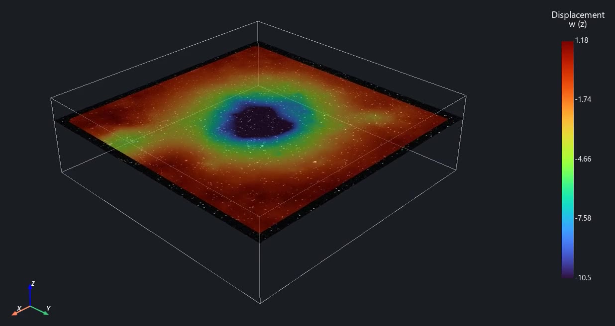
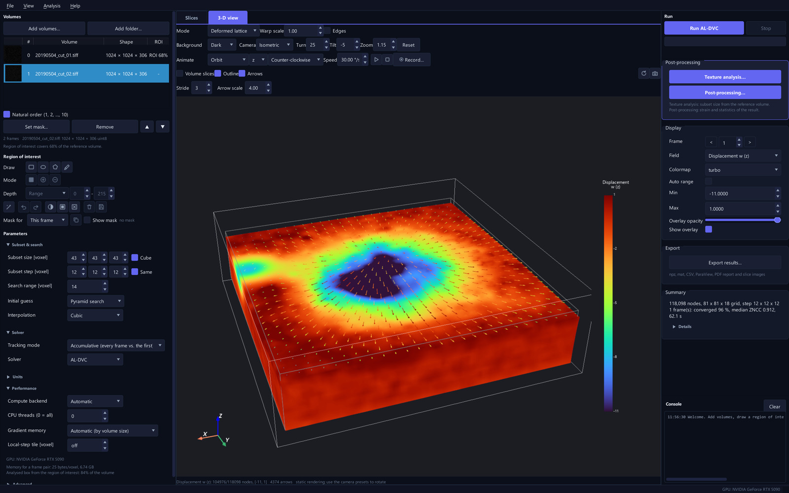
Sphere indentation of a hydrogel, confocal scan of 1024 × 1024 × 306 voxels. Colour: the vertical displacement w on the deformed node grid, with 3-D arrows; under the sphere w reaches −10.5 voxels. The node layers are drawn translucent, so colours blend where layers overlap. w, colour scale from purple to dark red:−10.5to+1.2 voxels Measured with pyALDVC, local subset solver The case
34s
on one NVIDIA RTX 5090 for a 1024 × 1024 × 306 confocal pair with 79,200 nodes (5.0 min on a 24-core CPU)
0.001–0.006voxel
displacement error on synthetic translation, rotation and 2 % strain
0.005–0.020voxel
median difference from the MATLAB ALDVC code on the same scan: 0.005 in u, 0.006 in v, 0.020 in w
14GB
volume memory of a masked 1024³ pair, from the memory model (was 53 GB)
1.2s
texture analysis of a 256³ volume
7
interface languages

Cases

Three data sets from the DVC Challenge 2.0 benchmark and one unpublished study. The foam, hydrogel and rotation animations were measured with pyALDVC and recorded in its 3-D view.

Case 1In-situ X-ray micro-CT

Foam under compression

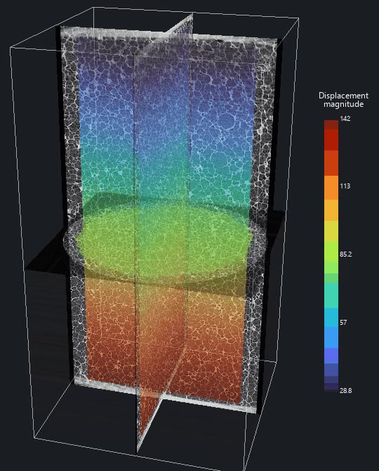
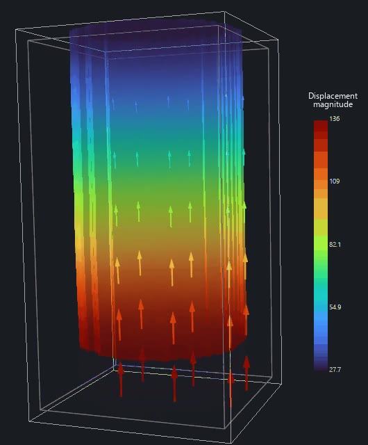
No speckle and no markers: pyALDVC follows the cell walls of an elastomeric closed-cell foam through 16-bit micro-CT volumes of 987 × 1009 × 1856 voxels. For the first compression step it measures the 3-D displacement on a 29 × 30 × 56 grid of 48,720 nodes, in a cylindrical region drawn on the slices. The field changes smoothly along the compression axis, and the slice sweep shows it on the cell walls themselves.

  • 1.8 billionvoxels per scan, 3.7 GB
  • 48,720grid nodes
  • ≈ 3 minon one GPU
Displacement magnitude in voxels over the micro-CT slices, swept through the specimen.
Displacement magnitude in voxels on the deformed node grid, with arrows; deformation exaggerated 2×, colour scale fitted to each frame.

First compression step. Measured with pyALDVC

Scan
4 µm voxels, 16-bit
Nodes
48,720 (29 × 30 × 56)
Subset / step
57 / 32 voxels
Solver
local subset
Frames
reference and first step
Hardware
one NVIDIA RTX 5090
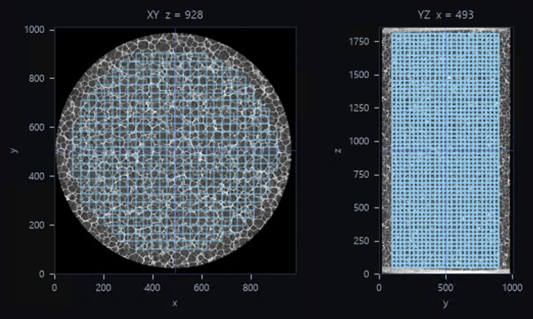
Two orthogonal grey-scale foam slices with a regular grid of blue node markers.
The node grid on the x–y and y–z micro-CT slices, inside the cylindrical region of interest (axes in voxels).
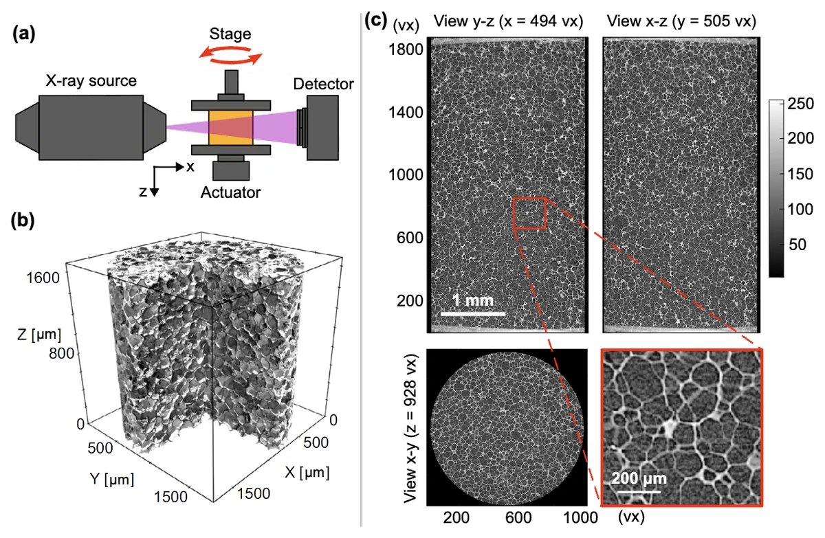
Figure: an X-ray CT loading stage, a 3-D rendering of the foam, and orthogonal grey-scale slices with a close-up of the cell walls.
The experiment: (a) loading stage between X-ray source and detector; (b) 3-D rendering; (c) orthogonal slices, 4 µm voxels, with a cell-wall close-up. Adapted from Tong et al. (2026, preprint); panel (b) after Landauer et al., Sci. Data (2023).
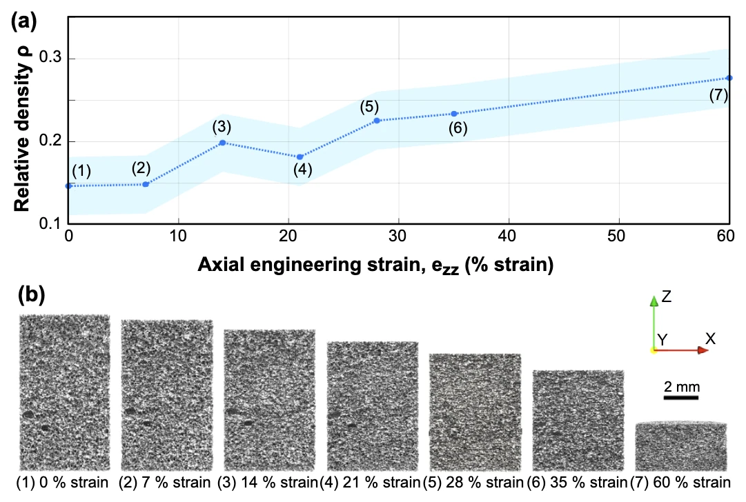
Figure: relative density plotted against axial strain, and seven vertical foam slices that are increasingly compressed.
Seven load steps from 0 to 60 % nominal compression: (a) relative density rises from about 0.15 to 0.28; (b) the central vertical slice at each step. Adapted from Tong et al. (2026, preprint), after Landauer et al., Sci. Data (2023). Data: NIST foam materials data framework, A. K. Landauer, O. L. Kafka, N. H. Moser and A. M. Forster (Landauer et al., Sci. Data 10, 356, 2023, doi:10.1038/s41597-023-02092-4), courtesy of NIST. Part of the DVC Challenge 2.0 dataset, doi:10.18434/mds2-4129.

Case 2Confocal microscopy

Hydrogel indentation

A sphere presses into a soft, transparent polyacrylamide hydrogel seeded with 1 µm fluorescent beads. From two confocal stacks of 1024 × 1024 × 306 voxels at 0.42 µm, pyALDVC measures the 3-D displacement at 144,342 nodes. The indentation dimple stands out: about 10.5 voxels (4.5 µm) of downward motion under the sphere, fading outward. The orbit at the top of the page shows the same field on the deformed node grid.

  • 144,342grid nodes
  • −4.5 µmw under the sphere, −10.5 voxels
  • 70.8 son one GPU
An x–y slice swept along z through the bead volume; the dimple under the sphere appears as the slice moves through the gel. Colour: vertical displacement w, −10.5+1.2 voxels Measured with pyALDVC
Scan
0.42 µm voxels (0.425 µm in z)
Nodes
144,342
Subset / step
43 / 12 voxels
Solver
local subset
Frames
reference and indented
Hardware
one NVIDIA RTX 5090
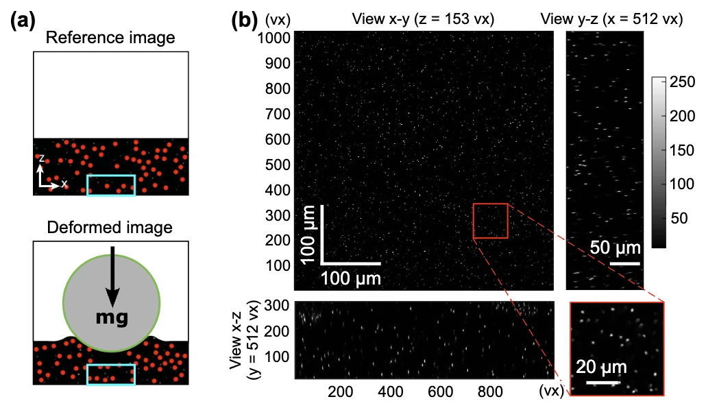
Figure: a schematic of a sphere indenting the gel, and confocal orthogonal views of fluorescent beads with a close-up.
The experiment: (a) reference and indented states; (b) confocal orthogonal views of the 1 µm fluorescent beads, 0.42 µm voxels, with a close-up. Adapted from Tong et al. (2026, preprint). Data: J. Yang, L. Hazlett, A. K. Landauer and C. Franck, the ALDVC example scans (Exp. Mech. 60, 1205–1223, 2020). Part of the DVC Challenge 2.0 dataset, doi:10.18434/mds2-4129.

Case 3Synthetic · incremental tracking

Rigid-body rotation

A synthetic bead volume of 512 × 512 × 192 voxels turns about the z axis in 5° steps up to 30°: points near the edge move tens of voxels, yet the true strain is exactly zero. pyALDVC tracks the six steps frame to frame. Its statistics tools fit such a rigid motion in closed form (a weighted Kabsch fit) and remove it, leaving the deformation and the measurement noise.

  • 30°in six 5° steps
  • ≈ 80voxels, largest u at 30°
  • 34 sall six steps, one GPU
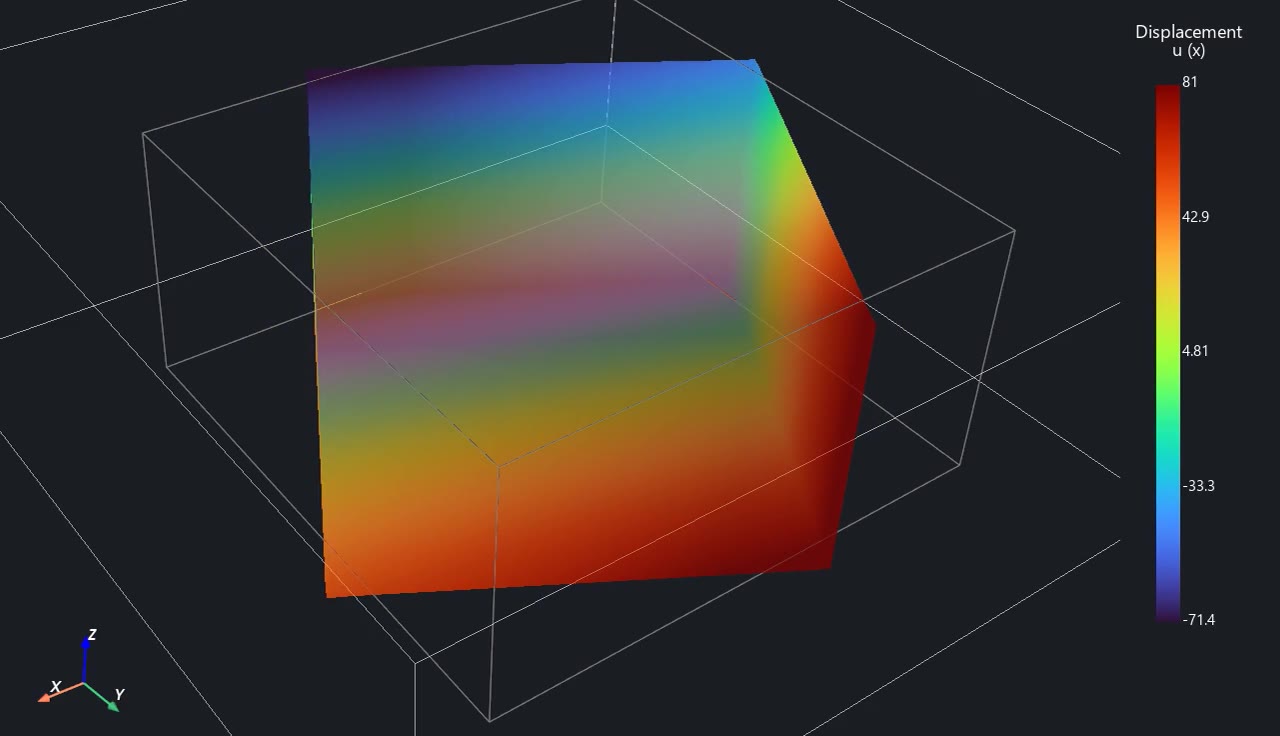
Horizontal displacement u in voxels on the deformed node grid as the volume turns from 0° to 30°, tracked frame to frame; the clip plays forward, then back, and the colour scale is fitted to each frame. Measured with pyALDVC
Scan
7 volumes, synthetic beads
Nodes
37,044 per frame
Subset / step
21 / 8 voxels
Solver
local subset
Tracking
incremental
Hardware
one NVIDIA RTX 5090

Data: synthetic bead volumes from the DVC Challenge 2.0 dataset, doi:10.18434/mds2-4129.

Case 4

Laser-induced cavitation

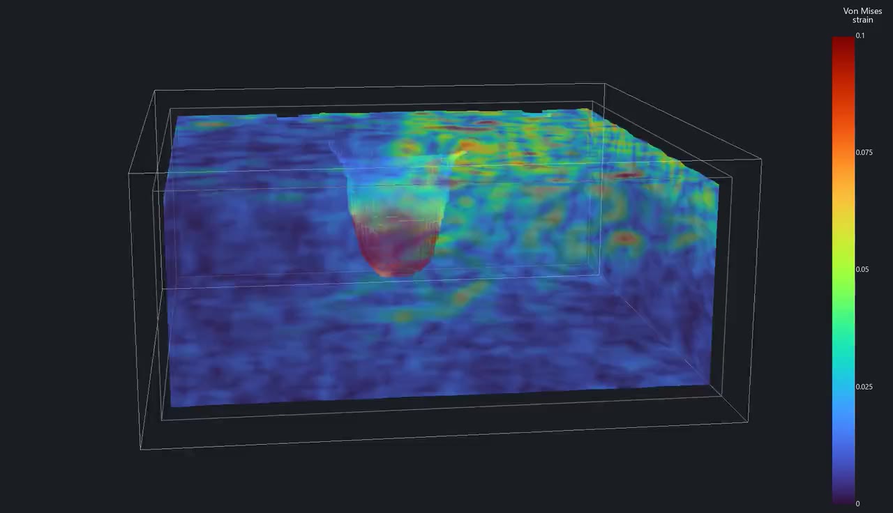
Residual von Mises strain left by laser-induced cavitation (unpublished data).

Subset sizes in the case settings are as entered in the application, which counts the odd span of a subset (2h + 1 voxels); the Python parameter winsize, the figures and the accuracy notes give the even edge 2h, one voxel less.

The foam, hydrogel and synthetic rotation data are part of the DVC Challenge 2.0 benchmark: Tong, Z. et al. Digital Volume Correlation Challenge 2.0: A Comprehensive Dataset for Digital Volume Correlation Benchmarking. Research Square preprint (2026), doi:10.21203/rs.3.rs-9683321/v1. Dataset: doi:10.18434/mds2-4129.

What it does

Everything between the scans and the exported field, in one application. The same functions are available from the command line and from Python.

  1. Point and click

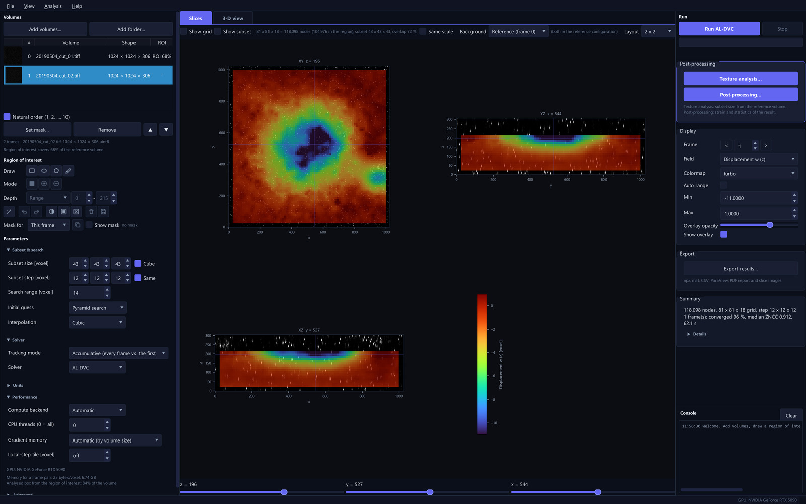
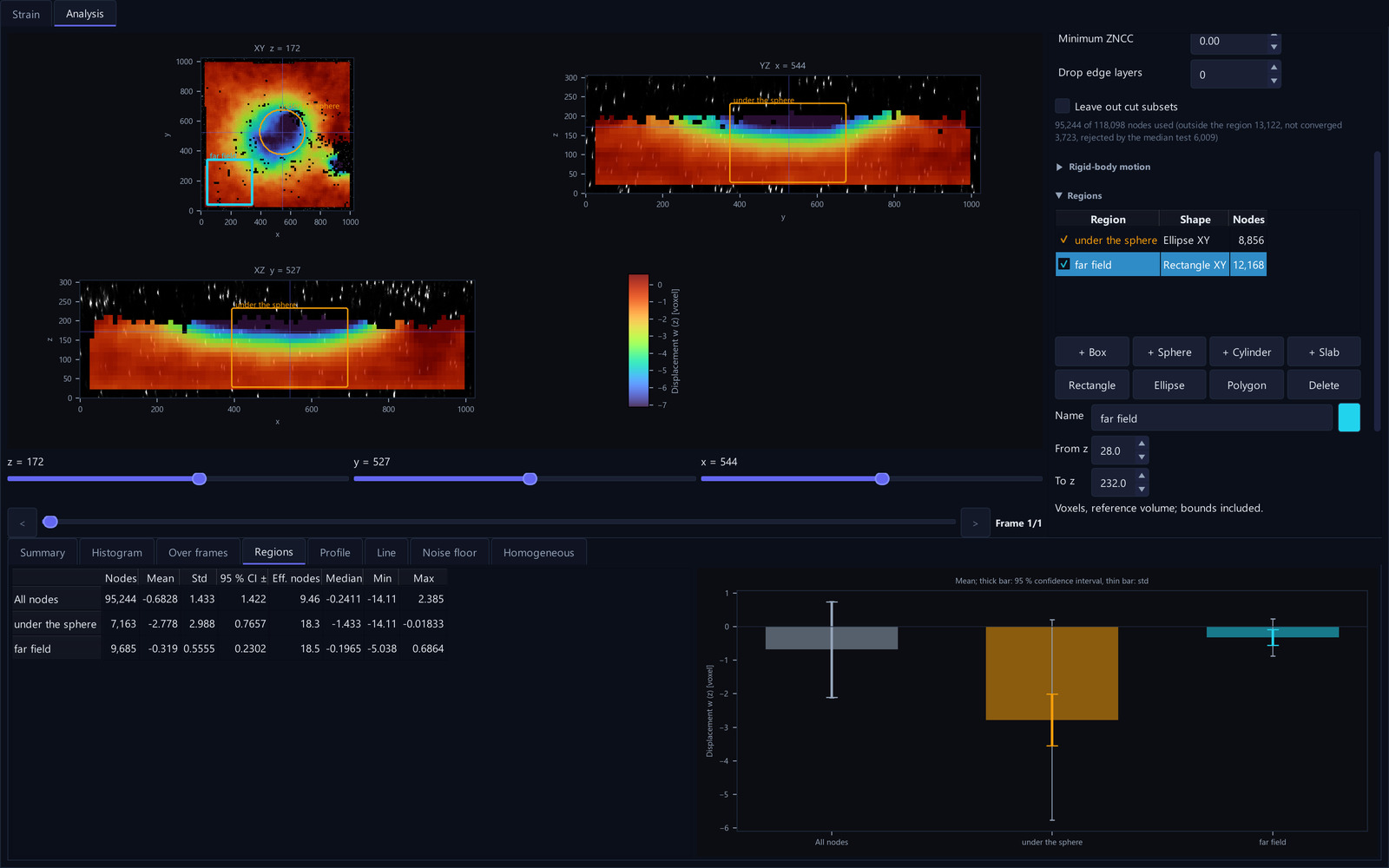
    Load the scans, draw the region of interest on the slices with a box, ellipse, polygon, brush or an automatic mask, run and export, in an interface available in seven languages.

    • English
    • 简体中文
    • 繁體中文
    • 日本語
    • Deutsch
    • Français
    • Español
  2. AL-DVC solver

    Local subset fits are coupled to one smooth, compatible displacement field, which gives cleaner gradients than subset DVC alone. Cracks and holes cut out of the region of interest split the subsets and the node grid, so the field is not smoothed across them (a crack front stays connected).

  3. NVIDIA GPU

    pip install "al-dvc[gpu]" runs the local solvers as CUDA kernels; their results typically differ from the CPU's by less than 10−5 voxel.

  4. Large volumes

    Streamed frames, gradients computed on the fly and local steps over sub-boxes keep the volume memory of a masked 1024³ pair at about 14 GB (memory model).

  5. Texture analysis

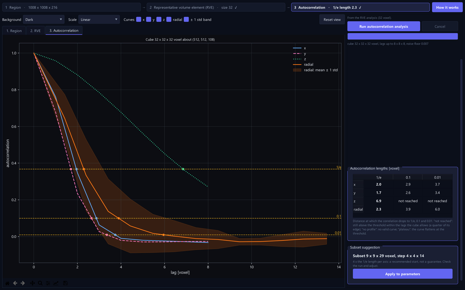
    Measures the correlation length and the representative volume of your scan and suggests a subset size and step, applied to the run with one click.

  6. Strain

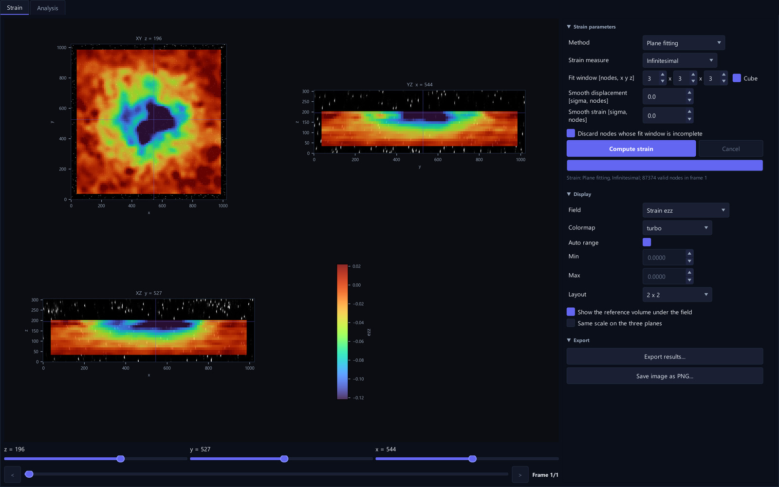
    Four gradient methods (plane fit, finite elements, finite differences, direct) and four measures (infinitesimal, Green–Lagrange, Euler–Almansi, Hencky), computed after the run in their own window.

  7. Statistics and rigid-body motion New in 0.10

    Means with 95 % confidence intervals, the noise floor, regions, profiles and a virtual extensometer, with the rigid-body motion fitted in closed form and removed.

  8. 3-D view and animations

    Field slices, the deformed node grid and displacement arrows, with orbits, frame sequences and slice sweeps recorded as GIF, or as MP4 with the optional imageio and imageio-ffmpeg.

  9. Formats

    Reads TIFF stacks and slice folders, MATLAB, NumPy and HDF5, and NIfTI, NRRD and DICOM with their optional readers (nibabel, pynrrd, pydicom); writes NumPy, MATLAB, CSV, ParaView and a PDF report.

  10. Sessions, batch and command line

    Save a session, queue sessions as a batch, resume long sequences from checkpoints, or run the same analysis with al-dvc or al_dvc.run_aldvc.

How it works

The method, and the tools that tell you how far to trust a result. The figures are computed from synthetic volumes with a known answer by a script in the repository, so they can be regenerated.

The augmented Lagrangian method

pyALDVC places a regular grid of nodes in the reference scan, each at the centre of a cubic subset, and solves two problems in turn. Local: each subset is matched to the deformed scan on its own, by an inverse-compositional Gauss-Newton fit of an affine warp (3 translations, 9 gradient terms) that minimises the zero-normalised sum of squared differences. This is precise where the texture is good, but the nodes are independent, so gradients are noisy and neighbours need not agree. Global: one smooth, kinematically compatible field is fitted to all local results with a finite-element solve. An augmented Lagrangian couples the two; three or four passes are enough, and the smoothness weight is chosen automatically.

Scans f, g reference and deformed Initial guess phase-correlation shift, then NCC on a pyramid Local fit, first pass 12 parameters per subset IC-GN on ZNSSD Weight β L-curve, once per reference ADMM LOOP · UP TO 4 GLOBAL STEPS Global step compatible field û: FEM + PCG Dual update W ← W + (∇û − F) v ← v + (û − u) Local fit, 3 parameters F fixed at ∇û, proximal μ term stop when the RMS update < 0.01 voxel Result U, F, ZNCC, U_std, status Strain, after the run 4 gradient methods × 4 measures Scans f, g reference and deformed Initial guess phase-correlation shift, then NCC on a pyramid Local fit, first pass 12 parameters per subset, IC-GN on ZNSSD Weight β L-curve, once per reference ADMM LOOP · UP TO 4 GLOBAL STEPS Global step compatible field û: FEM + PCG Dual update W ← W + (∇û − F) v ← v + (û − u) Local fit, 3 parameters F fixed at ∇û, proximal μ term stop when the RMS update < 0.01 voxel Result U, F, ZNCC, U_std, status Strain, after the run 4 gradient methods × 4 measures
Schematic 1 One run: an initial guess (a phase-correlation shift, then normalised cross-correlation on a pyramid), a 12-parameter local fit for every subset, then up to four ADMM passes in total (at most four global steps, each followed by a dual update and, while the loop goes on, a 3-parameter local fit), until the RMS update is below 0.01 voxel.
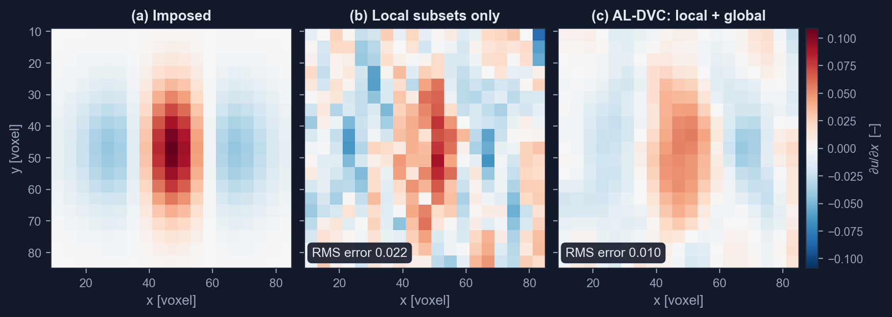
Three colour maps of ∂u/∂x: the imposed field, a noisy map from the local subsets, and a smoother map after the global step.
Figure 1 What the global step adds. The gradient ∂u/∂x of a smooth, localised displacement on the middle node layer of a noisy synthetic pair (SNR 2, subset 12 voxels): (a) imposed, (b) from the local subsets alone, (c) after the AL-DVC global step. The RMS error of ∂u/∂x falls from 0.022 to 0.010; the displacement error changes less, from 0.139 to 0.121 voxel. Over three noise seeds the error of the full gradient is 2.4–2.5 times lower after the global step.

Tracking a sequence

A sequence of scans can be tracked two ways. Accumulative (the default): every scan is correlated with the first, so errors do not add up from step to step. Incremental: every scan is correlated with the one before, and the steps are chained back to the first scan by interpolating each step's displacement at the points' current positions. Incremental tracking follows deformations too large for a subset to still match its first-scan appearance, at the cost of a small error per step; the rotation case above was tracked this way. Every pair starts from a coarse-to-fine guess: a phase-correlation shift, then normalised cross-correlation on a pyramid of downsampled scans, with the search widened when many peaks hit its edge.

Accumulative every scan against scan 0 (the default) Incremental every scan against the one before 0 1 2 3 4 0 1 2 3 4 chained back to scan 0: each step interpolated at the tracked positions (cubic) Accumulative (the default) every scan against scan 0 0 1 2 3 4 Incremental every scan against the one before 0 1 2 3 4 chained back to scan 0: each step interpolated at the tracked positions (cubic)
Schematic 2 Accumulative: every scan against scan 0. Incremental: every scan against the previous one, chained back to scan 0 by cubic interpolation at the tracked positions.
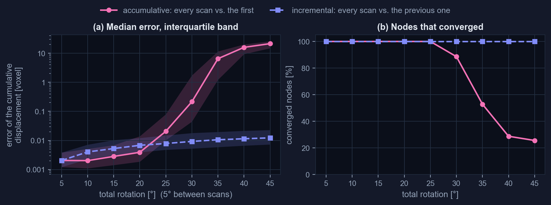
Two charts against total rotation: the accumulative error rises steeply after 20° and its share of converged nodes drops, while the incremental curves stay flat.
Figure 2 Accumulative against incremental tracking of a speckled cylinder turning 5° between scans (synthetic, subset 16 voxels). (a) Accumulative tracking keeps a median error of 0.004 voxel or less up to 20°, then degrades and breaks down beyond 25°; (b) 88.6 % of its nodes converge at 30° and 29 % at 40°. Incremental tracking converges at every node evaluated up to 45°, its median error growing slowly from 0.002 to 0.012 voxel. Where accumulative tracking fails depends on the subset size and the texture.

Texture analysis in three steps

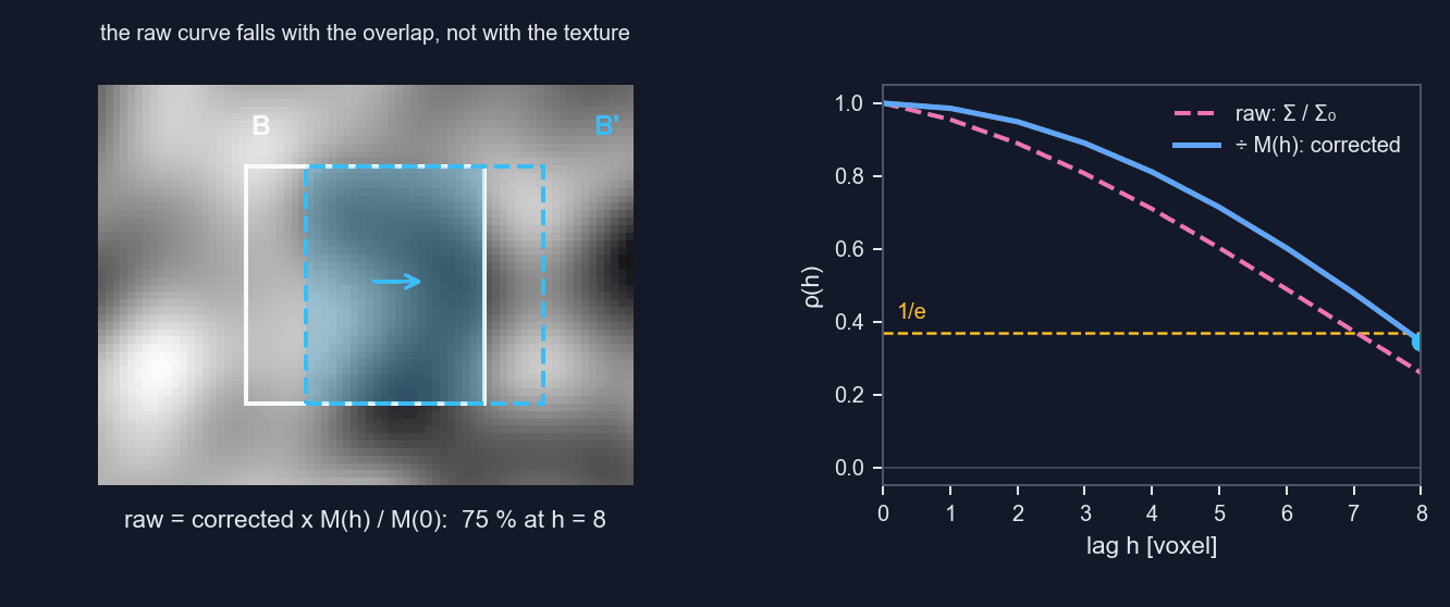
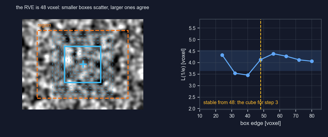
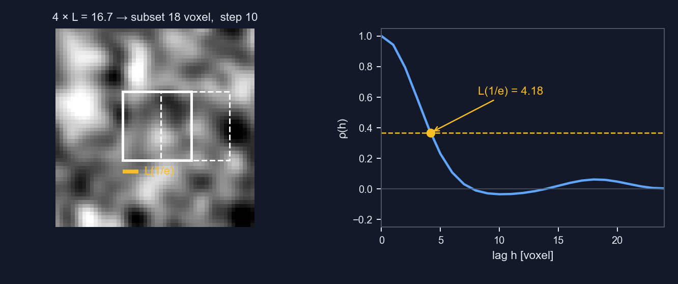
A subset can only be followed if it holds enough texture: several speckles, beads or cell walls. The texture analysis measures how far grey values stay correlated and turns that into a subset size. 1. Correlation length. Compare a cube with shifted copies of itself; the shift at which the correlation falls to 1/e is the correlation length. Each value is divided by the number of voxel pairs that still overlap, so the shrinking overlap does not bias it. 2. Representative volume. Grow the cube about one centre until the length stops changing. 3. Subset. Suggest four correlation lengths per axis and a step of half a subset: a starting point, applied with one click.

Step 1 A cube and its shifted copy. The overlap shrinks as the shift grows, so the raw correlation falls faster than the overlap-corrected one.
Step 2 Concentric cubes of growing size about one centre. The correlation length settles once the cube is larger than the representative volume.
A speckle image with a subset box about four correlation lengths wide and its copy one step along, next to a correlation curve crossing 1/e.
Step 3 From the 1/e correlation length to the subset: four lengths, rounded up to an even edge, and a step of half the subset, also even.
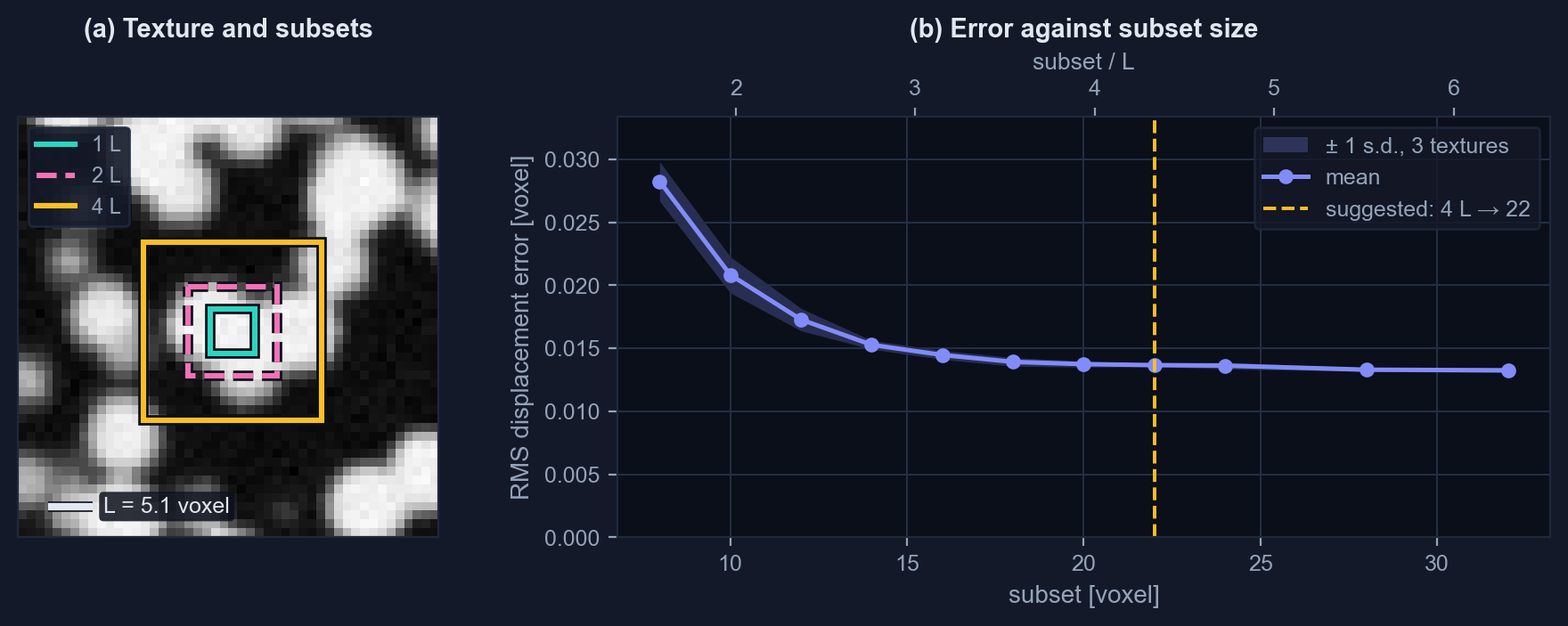
A grey-scale texture of bright spheres with nested boxes of one, two and four correlation lengths, and a curve of displacement error against subset size that falls steeply and flattens near the suggested size.
Figure 3 Why four lengths. (a) A synthetic texture of random spheres with a correlation length L of 5.1 voxels, and subsets of 1, 2 and 4 L. (b) The displacement error over three such textures falls from 0.028 voxel at the smallest subset, 8 voxels, to 0.0137 at the suggested 22 voxels (four per-axis lengths, rounded up to an even edge), and barely changes with larger subsets (0.0133 at 32). Noisy scans may need larger subsets, finely varying fields smaller ones.

How precise is the result?

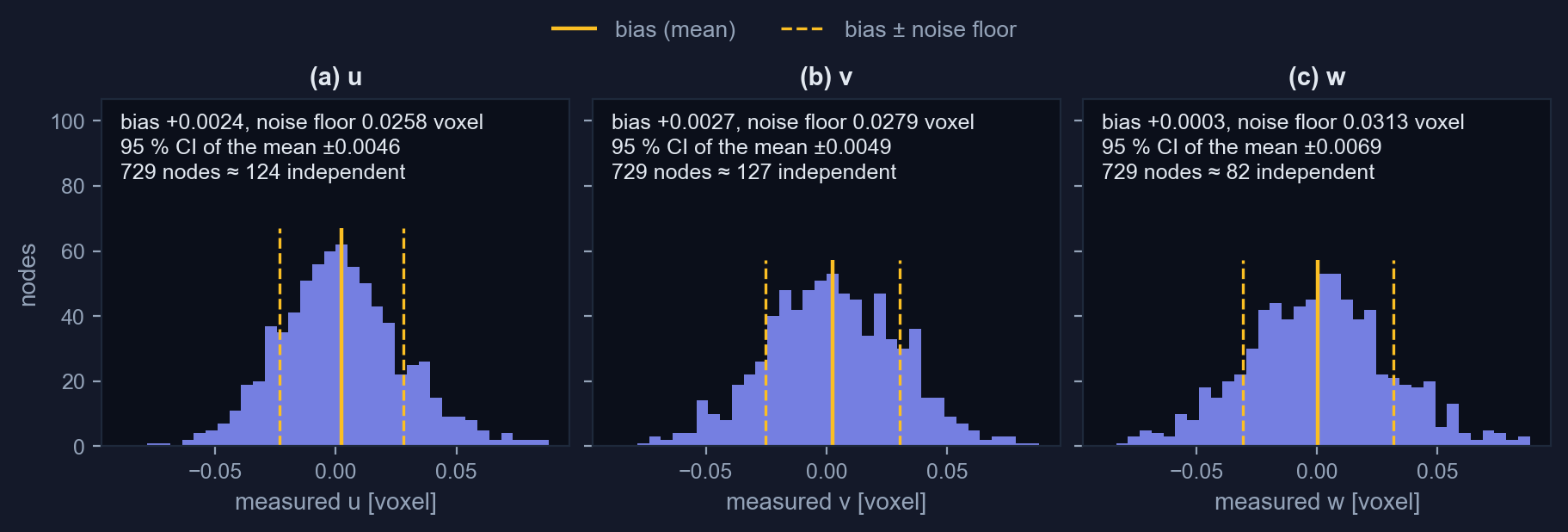
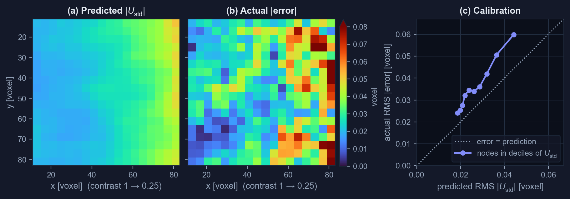
pyALDVC reports precision in three ways. Noise floor: for two scans of a static specimen, or a known translation, it uses the DVC Challenge 2.0 definitions: the bias is the mean error of each component, the noise floor its population standard deviation after that mean is removed, and urms combines both; MAER/SDER, the virtual strain gauge and, for several static scans, spatial and temporal noise are reported too. Per node: every converged node carries Ustd, a standard deviation of its local subset fit, predicted from its own residual and Gauss-Newton matrix at no extra cost. Means: every mean comes with a 95 % confidence interval built on the effective number of independent nodes, because overlapping subsets make std/√N far too optimistic.

Three histograms of measured u, v and w for a static pair, each centred near zero, with a solid line at the bias and dashed lines one noise floor either side.
Figure 4 Two scans of a static specimen (synthetic, 8-bit, independent noise of 2 % of full scale in each): measured (a) u, (b) v and (c) w, with the bias (solid line) and the bias ± noise floor (dashed); urms is 0.049 voxel. The 729 nodes are worth about 124 independent values for u, so the 95 % interval of its mean is ±0.0046 voxel, 2.45× wider than the naive ±0.0019.
Two maps, predicted and actual displacement error, both growing towards the low-contrast side, and a calibration curve lying above the identity line.
Figure 5 Predicted against actual error where the texture contrast fades from 1 to 0.25 along x (synthetic): (a) Ustd from the run, (b) the actual error of the local subset fit, (c) calibration over deciles of Ustd. The error grows where Ustd does, but the prediction runs low: 68–80 % of the actual error per decile, 74 % overall. Ustd describes the local fit and assumes similar noise in both scans; the global step lowers the error of the final field.

Removing rigid-body motion

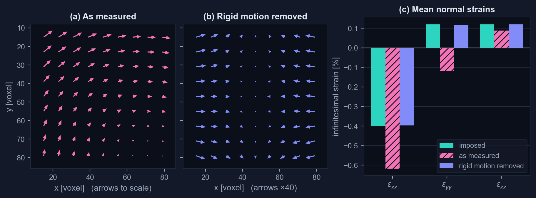
A specimen that shifts or turns between scans adds displacement that is not deformation, and a rotation even reads as false infinitesimal strain: 2° gives about −6 × 10−4. pyALDVC removes a translation (the mean, as the DVC Challenge 2.0 noise floor does), a rigid motion, or the whole affine part. The rigid fit is a closed-form, weighted Kabsch solution in physical units, and it can be fitted over one region, such as a grip, and removed everywhere. Strain is recomputed from the corrected gradient, RT(I + H) − I: the Green–Lagrange strain is unchanged, the infinitesimal strain loses the rotation. The stored result is never edited; the corrected field can be shown and exported, with its fit recorded.

Arrow plots before and after removing the rigid motion, and a bar chart in which the corrected normal strains match the imposed ones.
Figure 6 A 4° rotation about an oblique axis and a translation, on top of a small compression along x with Poisson expansion (synthetic). (a) As measured, the rotation dominates the arrows and distorts the infinitesimal strains. (b) With the fitted rigid motion (4.00°) removed, the compression and the expansion appear (arrows ×40). (c) Mean εxx / εyy / εzz: imposed −0.40 / +0.12 / +0.12 %, as measured −0.62 / −0.12 / +0.09 %, with the rigid motion removed −0.397 / +0.116 / +0.119 %.

Accuracy and speed

Synthetic volumes with a known deformation, and the confocal hydrogel scan run through both pyALDVC and the MATLAB ALDVC code.

Accuracy and speed of pyALDVC
TestResult
Rigid translation, synthetic0.003–0.006 voxel
2 % strain, synthetic0.004 voxel
5° rotation, synthetic0.001 voxel
Translation by (12.3, −9.6, 7.4) voxels plus 1 % strain, synthetic0.004–0.005 voxel
2 % strain, noisy scan (SNR 6)0.011–0.012 voxel
The confocal hydrogel pair against MATLAB ALDVCmedian difference 0.005 / 0.006 / 0.020 voxel (u, v, w)
GPU against CPUtypically below 10−5 voxel

Synthetic rows: RMS error of each displacement component at the interior nodes, subset 16, step 8 voxels. MATLAB row: subset 32, step 8 voxels, 79,200 nodes. These subsets are the Python winsize; the application shows one voxel more (17 and 33). The difference in w is larger mainly because the confocal scan has far less texture along z, where both codes stop early; the two codes also reject different outliers. The synthetic rows use the default settings; the MATLAB row and the timing use the settings of the MATLAB example run, so both codes solve the same problem. Every push to the main branch is tested on Python 3.10, 3.11 and 3.12.

Get started

Install

conda create -n pyaldvc python=3.12 -y
conda activate pyaldvc
pip install al-dvc    # NVIDIA GPU: pip install "al-dvc[gpu]"
al-dvc                # opens the application

conda only provides Python here: al-dvc and its dependencies come from PyPI.

The GPU flavour needs an NVIDIA driver, not the CUDA Toolkit.

Copy leaves the comments out, so the lines run as they are in Anaconda Prompt, PowerShell or a Unix shell.

To update: pip install --upgrade al-dvc, or pip install --upgrade "al-dvc[gpu]" for the GPU flavour. Your settings are kept.

No Python?

Every release ships a portable Windows bundle: unzip it and double-click pyALDVC.exe. The bundle runs on the CPU.

Download for Windows

Check the install

al-dvc --self-test runs six checks, prints [ok] or [FAIL] for each and saves them to pyaldvc_self_test.txt. The compute-backend line names the GPU when one is used.

Learn

The user guide covers data preparation, parameters, results, statistics, exports, the GPU and the command line.

Read the user guide

Cite

If pyALDVC helps your research, please cite the software and the method.

Software

Tong, Z., Yang, J. pyALDVC: Augmented Lagrangian Digital Volume Correlation in Python. Zenodo (2026). doi:10.5281/zenodo.22883767

The concept DOI always resolves to the latest release; each release also has its own DOI.

Method

Yang, J., Hazlett, L., Landauer, A. K., Franck, C. Augmented Lagrangian Digital Volume Correlation (ALDVC). Experimental Mechanics 60, 1205–1223 (2020). doi:10.1007/s11340-020-00607-3

BibTeX
@software{tong_pyaldvc,
  author    = {Tong, Zixiang and Yang, Jin},
  title     = {{pyALDVC}: Augmented Lagrangian Digital Volume Correlation in Python},
  publisher = {Zenodo},
  year      = {2026},
  doi       = {10.5281/zenodo.22883767},
  url       = {https://github.com/zachtong/pyALDVC}
}

@article{yang_aldvc_2020,
  author  = {Yang, Jin and Hazlett, Lauren and Landauer, Alexander K. and Franck, Christian},
  title   = {Augmented {Lagrangian} Digital Volume Correlation ({ALDVC})},
  journal = {Experimental Mechanics},
  volume  = {60},
  number  = {9},
  pages   = {1205--1223},
  year    = {2020},
  doi     = {10.1007/s11340-020-00607-3}
}

Using the case data? Cite the DVC Challenge 2.0 dataset (doi:10.18434/mds2-4129) and paper (Tong et al., Research Square preprint, 2026, doi:10.21203/rs.3.rs-9683321/v1) and, for the foam, Landauer et al., Sci. Data 10, 356 (2023).